Overview
It is hard to understate the importance of Google Earth Engine (GEE) as a repository of remote sensing and climate data. Truly, there are thousands of collections including what I would consider one of the greatest gifts the United States has bestowed upon humanity, the Landsat collection. GEE has all the imagery from Landsat 4 through Landsat 9 which represents more than 40 years of imagery to analyze change on our home planet. Also in the collection is the Landsat Global Land Survey of 1975 which is a compilation of scenes created by Landsat 1 through Landsat 3 MSS sensors. In this very short tutorial, I will demonstrate how I access this imagery and create functions by which I can quickly and efficiently process large amounts of data.
I tend to use GEE to rapidly prototype ideas and thoughts in an effort to see those ideas “fail rapidly” before I invest the time to develop operational code to process imagery in the operational context using on-premises servers. So let’s dig right in and start coding up a simple script which at the end will display a Sentinel-2 scene on a date and location specified by the code and position of the GEE Map and also produce several typical normalized band indices.
Setting up our global variables
Although Landsat does give us 41 years of continuous observations within the GEE library, I tend to use Sentinel-2 imagery for recent observations due to its reduced re-visit time which offers more chances of cloud free imagery over the area I am studying. First question we need to ask, what period of time do we need to study? Let’s assume for this example, we want the latest image because we want to see the effects of flooding, snowfall, turbidity, etc.
// Set Variables
var begin_date = '2024-11-18';
var end_date = '2024-11-30';
var map_center = Map.getCenter():
var cloud_percent_max = 40;
GEE’s web interface uses Javascript. But you can interface with GEE through R and RShiny Apps, Python, and Python Jupyter Notebooks, QGIS, etc. So far, we have instantiated 4 client side objects that will be used to filter the Sentinel-2 library to a manageable number of images. We will filter by date, we will only select those images which intersect the center of our map display, and finally we filter out the worst of the cloudy images.
Selecting our ImageCollection and Filtering
// Retrieve the Image Collection
var s2 = ee.ImageCollection('COPERNICUS/S2_SR_HARMONIZED')
    .filterBounds(map_center)
    .filter(ee.Filter.lt('CLOUDY_PIXEL_PERCENTAGE', cloud_percent_max))
    .filterDate(begin_date, end_date);
So, when this code is executed, we create a server side Image Collection which is filtered using the criteria we set (location, cloudiness, and dates). The images inside this collection are stored on Google servers with their Digital Number (DN) values. We want Bottom of Atmosphere values so we need to convert the DN to a float by multiplying each image by the scaling factor of 1/1000. The ‘S2_SR_HARMONIZED’ data is atmospherically corrected data and was processed by Sen2Cor software. If you need specific atmospheric correction, you should use the S2_HARMONIZED collection and apply the correction through your code.
To modify image collections, we need to ‘map’ the image collection through a function, which will apply the process in the function to each image.
Functions
To create a function, you need to instantiate it with a variable name, it’s input(s), then the processing that will occur on the input(s), and define what the returned object will be. For our first function, let’s convert the DN values to scaled values:
var convert_from_dn = function(image) {
    return(image.multiply(0.001).copyProperties(image));
};
That is about as simple as a function you will find. In the return statement you will notice that I appended .copyProperties(image) to the end of the math portion. I do that to preserve the metadata that was originally in the ImageCollection. Without it, the metadata is stripped off.
Next, let’s ensure all of the bands in our ImageCollection have the same spatial resolution, to avoid the odd artifacts that occur when we you apply raster math to images in GEE with different cell sizes. To do this we will create another function:
var resample_20m = function(image) {
    var projection = image.select('B11').projection();
    var resample = image.reproject({
        crs: projection,
        scale: 20
    });
    return(resample.copyProperties(image));
};
Finally, lets create a simple function by which we can efficiently create normalized difference indices. GEE has an function for calculating normalized difference for images called ee.Image.normalizedDifference() but we are working with an ImageCollection. We’ll need to map that function, and we might as well write the function so that it is mutable and can be used to create any normalized difference product – say we want a Normalized Difference Vegetation Index, Modified Normalized Difference Water Index, and Normalized Difference Turbidity Index.
var normalized_index = function(reflector, absorber, name) {
    var nested_func = function(image) {
        var ndi = image.normalizedDifference([reflector, absorber])
            .rename(name)
            .copyProperties(image);

        };

    return(nested_funct);
};
The normalized_index function seems to be much more complex that what we’ve used so far. But it’s still pretty simple when you understand why we need to write it this way. Typically, when we map a function against an ImageCollection, the server only accepts one input to the function and that’s the images in the ImageCollection. But in this instance, we really need to have multiple inputs. We need an input to define which band preferentially reflects for the phenomena we are mapping (NIR for plants) and which band is preferentially absorbed for the phenomena we are mapping (Red for plants). We also want to rename the image to something descriptive. To get around the single input limitation, we create a nested function where the outside function contains the band names and the inside function contains what happens to the individual images mapped to it.
Functions defined, let’s map the image collection to the functions.
So far we have all our functions we feel necessary to view Sentinel-2 imagery and a few simple derived Sentinel-2 analysis products. Those functions are not doing anything until we actually map the ImageCollection to them. So, let’s add to the variable s2 we defined earlier and append our mapping to it.
var s2 = ee.ImageCollection('COPERNICUS/S2_SR_HARMONIZED')
    .filterBounds(map_center)
    .filter(ee.Filter.lt('CLOUDY_PIXEL_PERCENTAGE', cloudy_percent_max))
    .filterDate(begin_date, end_date)
    .map(covert_from_dn)
    .map(resample_20m)
    .map(normalized_index('B8', 'B4', 'NDVI'))
    .map(normalized_index('B3', 'B11', 'MNDWI'))
    .map(normalized_index('B4' , 'B3', 'NDTI'))
    .sort('CLOUDY_PIXEL_PERCENTAGE').first();
In this example, we are adding three bands to the ImageCollection: Normalized Difference Vegetation Index (NDVI), Modified Normalized Difference Water Index (MNDWI), and Normalized Difference Turbidity Index (NDTI). At the end, I sorted the returned image collection by cloudiness, with the most cloud free image in the date range first. Note that the functions which are not nested convert_from_dn and resample_20m do not have any arguments assigned to them, only the normalized_index has that requirement in this example.
That’s it, we are ready to view the results!
Map Visualization
Each Map.addLayer() call adds a layer in order, from top down. So, let’s begin by using the Sentinel-2 image, visualized with false-color to enhance vegetation and water turbidity. We’ll place the NIR (Band 8) in the Red Channel, Red (Band 4) in the Green Channel, and Green (Band 3) in the Blue Channel .Map.addLayer(s2, {bands:['B8', 'B4', 'B3'], min:0, max:2.5}, 'S2 False-Color');
The {} in that line of code represent how we want to symbolize the result on the map. We’re declaring an RGB product by using the ‘bands’ input, with which bands in order as a list, and the minimum and maximum values by which to apply the histogram stretch to the image. Frequently, the min/max values will require a little experimentation to get the amount of contrast and aesthetic you are looking for. If we make our selection dates (2024-11-01 to 2024-11-30) using the above variables and placing the center of the map on the the mouth of the Mississippi River we should see this:
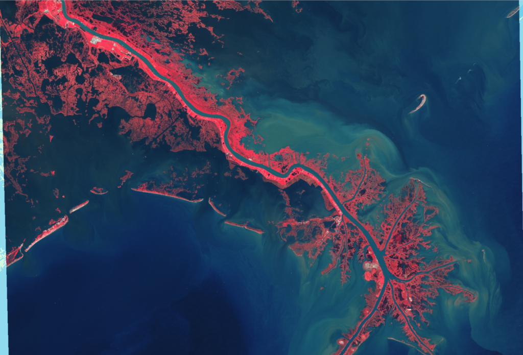
That turbidity in the outflow is rather beautiful and we have a turbidity index in the code, so let’s visualize it. But, we first need to consider that the turbidity index isn’t very useful over land features. So, we need to display the NDTI, but only over water. We can do that by creating a ee.image.updateMask() to limit the NDTI only over water. We have our Modified Normalized Water Index, so let’s first find out what values correspond to water in the MNDWI.Map.addLayer(s2.select('MNDWI'), {min:-0.5, max:0.5, palette:['green', 'yellow', 'blue']}, 'MNDWI');
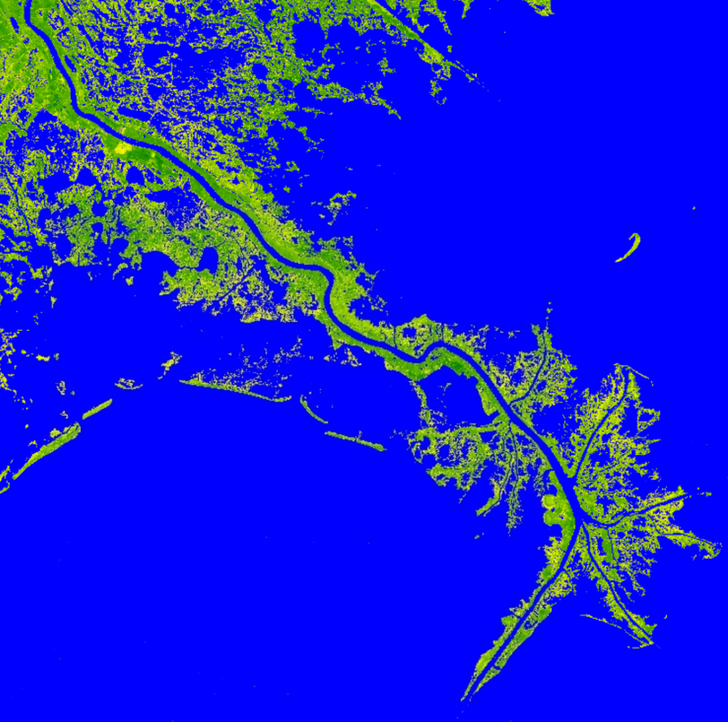
Notice, this time, because MNDWI is a single raster image, we don’t use ‘bands’ inside the brackets for the visualization, but rather a list of colors with the palette entry. GEE will smoothly blend those colors into a gradient to help you visualized the difference of values pixel by pixel. The MNDWI analysis is typically very sensitive to water, which explains the homogeneity of blue in the image. By, clicking the “Inspector” tab in the upper right of the GEE page, we can click with our mouse in to find the smallest, most isolated water, where the reflectance and absorption profile for SWIR and Green bands would be the most influenced by non-water features. Zooming into the false-color image onto a small bayou, I find a pixel I want to interrogate.
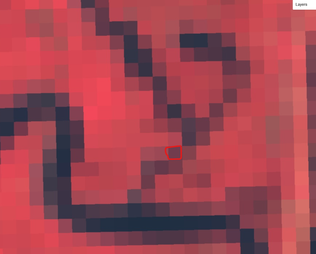
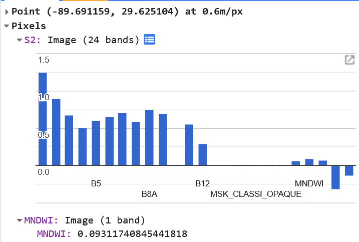
According to this, positive values seem to correlate with water features. But, for the sake of safety, let’s add a buffer to that idea and err on the side of underclassifying water features by using an MNDWI value of 0.2. We’re going to use that value to mask out the land in the NDTI analysis.var ndti = s2.select('NDTI');ndti = ndti.updateMask(s2.select('MNDWI').gt(0.2);
Let’s visualize that result:Map.addLayer(ndti, {min:-0.25, max:0.25, palette:['blue', 'green', 'yellow', 'brown']}, 'NDTI');
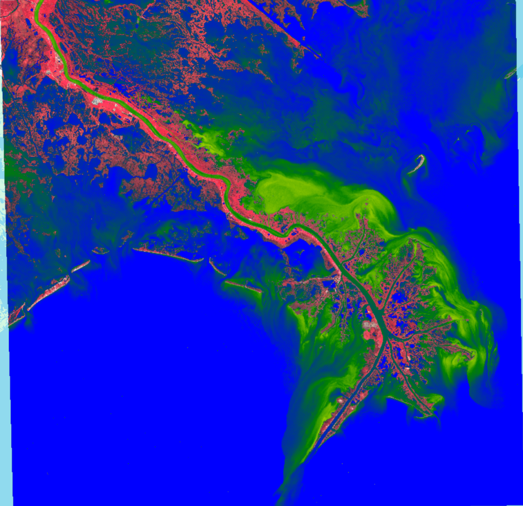
The bright blues show where the water doesn’t have many particulates and the normalized difference between Red and Green bands on the Sentinel-2 image are less than -0.25. We don’t see much if any brown colors, so the turbidity index generally stays below a positive value of 0.25. We can clearly see the relative density of sediments in the water around the mouth of the river and the effects of the current on those sediments.
Summary
Hopefully, this gentle tutorial helped you get on the path of accessing and preparing data to be viewed in Google Earth Engine. When working with ImageCollections, it’s always important to remember to map your indices and algorithms to the collection using functions. In future installments, we will tackle the various ways of masking out clouds from the images. But first, we need to be able to get the data, and get it ready.
The Full Code:
// SET VARIABLES
var begin_date = '2024-11-01';
var end_date = '2024-11-30';
var map_center = Map.getCenter();
var cloudy_percent_max = 40;

// FUNCTIONS and TOOLS
var convert_from_dn = function(image){
  return(image.multiply(0.001).copyProperties(image));
};

var normalized_index = function(reflector, absorber, name) {
  var nested = function(image){
    var ndi = image.normalizedDifference([reflector, absorber])
      .rename(name)
      .copyProperties(image);
    return(image.addBands(ndi))
  };
  return(nested);
};

var resample_20m = function(image) {
    var projection = image.select('B11').projection();
    var resample = image.reproject({
      crs: projection,
      scale: 20
    });
    return(resample.copyProperties(image));
};


// RETRIEVE THE IMAGE
var s2 = ee.ImageCollection('COPERNICUS/S2_HARMONIZED')
  .filterBounds(map_center)
  .filter(ee.Filter.lt('CLOUDY_PIXEL_PERCENTAGE', cloudy_percent_max))
  .filterDate(begin_date, end_date)

  .map(convert_from_dn)
  .map(resample_20m)
  .map(normalized_index('B3', 'B11', 'MNDWI'))
  .map(normalized_index('B4', 'B3', 'NDTI'))
  .sort('CLOUDY_PIXEL_PERCENTAGE').first();


print(s2);

var mndwi = s2.select('MNDWI');
var ndti = s2.select('NDTI');

ndti = ndti.updateMask(mndwi.gt(0.2));

Map.addLayer(s2, {bands:['B8', 'B4', 'B3'], min:0, max:2.5}, 'S2');
Map.addLayer(mndwi, {min:-0.5, max:0.5, palette:[ 'green', 'yellow', 'blue']}, 'MNDWI', false);
Map.addLayer(ndti, {min:-0.25, max:0.25, palette:['blue', 'green', 'yellow', 'brown']}, 'NDTI');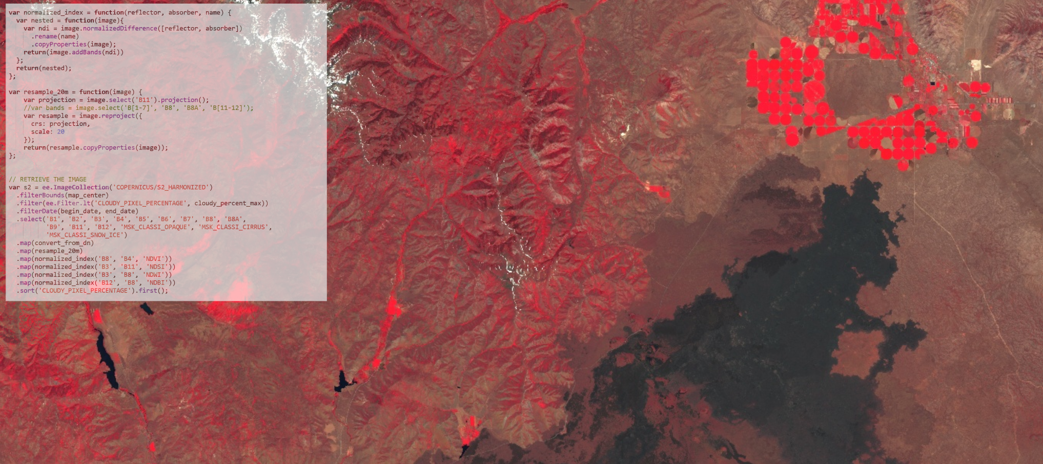
No responses yet